Balancing Car
Table of Contents
A self-balancing two-wheel robot on a LinkIt 7697 — state-space control, IMU sensor fusion, and a small reinforcement-learning model.
This is a project about the self-balancing car.
From 2017 — the control-theory and embedded-systems foundation (state-space models, sensor fusion, real-time control loops) that later led into the middleware layer under ROS 2. See the write-up in the CV, or the code at balancing-robot.
ROBOTS
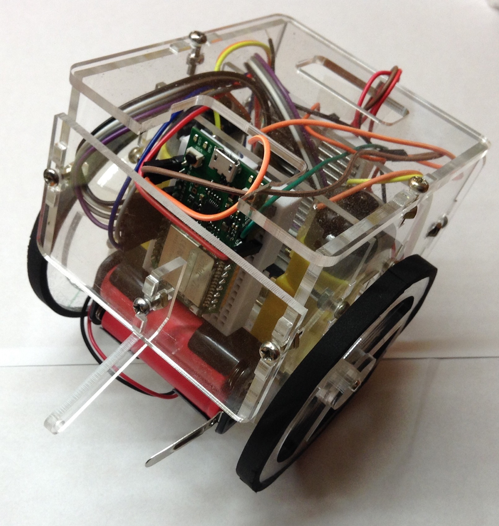
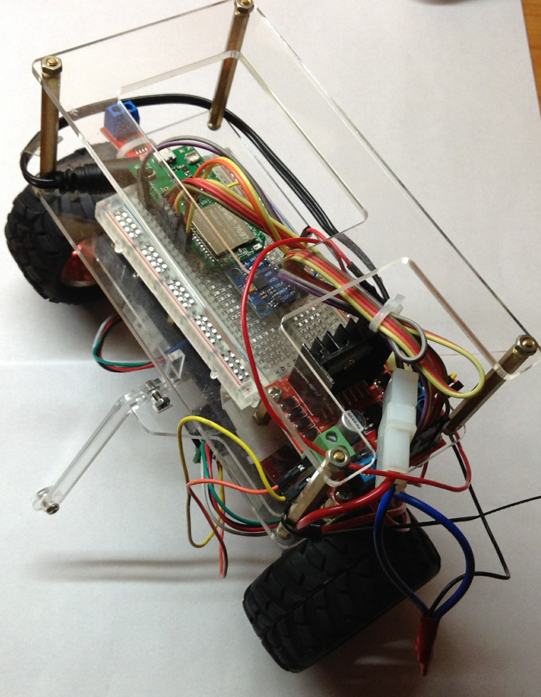
There are two version of robot car, right one is is 1st ver. robot car in big size, operating in 12V, but since it's so bulky to balance itself, so there is the 2nd ver. in small size, which is small, compact, modularized and easy to train and verified the control theorem.
PHYSICAL MODEL
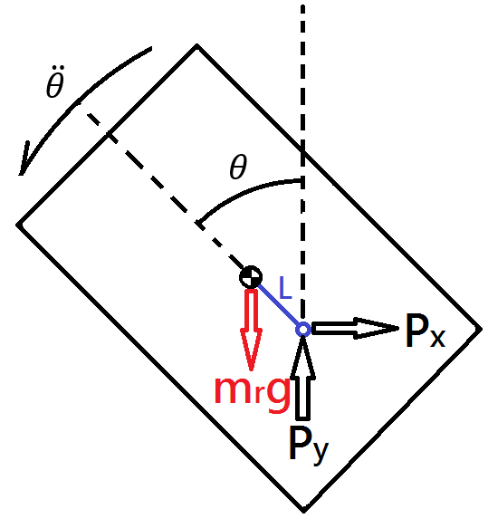
The robot which is equivalent to an inverted pendulum consists of two parts, the rod and the wheel. The goal is to drive the wheel properly to prevent tilting, so we have to calculate the relative inertial force caused by the acceleration of wheel.
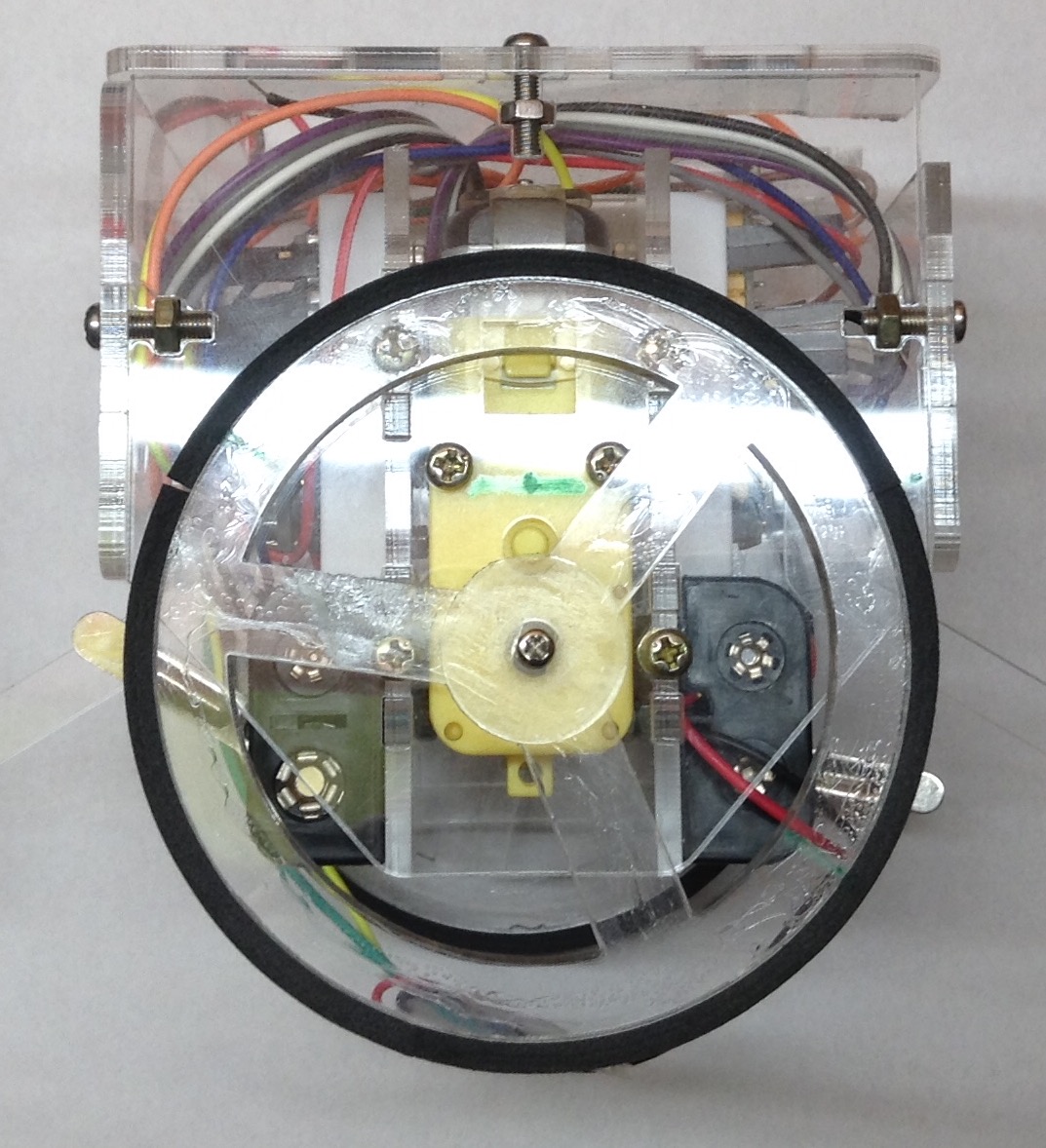
Following pictures are the Free Body Diagram of the two parts, rod and wheel.
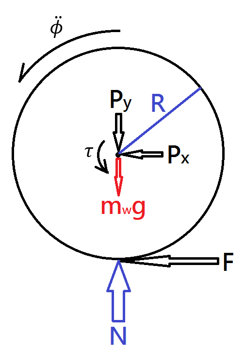
There are two methods to deal with the model, one is the classical way in Newton Physics, another one is using Lagrangian method, i.e. energy method.
NEWTON METHOD
Angular acceleration of wheel
$$I\omega \ddot{\phi}=\tau -F\cdot R$$
Linear acceleration of wheel C.M.
$$\hat{i}:m_w \cdot\ddot{x}=-P_x-F$$
$$\hat{j}:0=N-P_y-m_wg$$
Angular acceleration of rod
$$I_r\ddot{\theta}=-\tau + P_yL\sin \theta+P_xL\cos \theta$$
Linear acceleration of rod C.M.
$$\begin{align} \hat{i}&:m_r(\ddot{x}-\ddot{\theta}L\cos\theta+\dot{\theta}^2L\sin\theta)=P_x \ \cos\theta \hat{i}+\sin\theta \hat{j}&:m_r(\ddot{x}\cos\theta-\ddot{\theta}L)=-m_rg\sin\theta+P_y\sin\theta+P_x\cos\theta \end{align}$$
Position of C.M. of rod
$$r=x\hat{i}-L\sin\theta\hat{i}+L\cos\theta\hat{j}$$
Velocity of C.M. of rod
$$\dot{r}=\dot{x}\hat{i}-\dot{\theta}L\cos\theta\hat{i}-\dot{\theta}L\sin\theta\hat{j}$$
Acceleration of C.M. of rod
$$\begin{align} \ddot{r}&=(\ddot{x}-\ddot{\theta}L\cos\theta+ \dot{\theta}^2L\sin\theta)\hat{i}-(\ddot{\theta}L\sin\theta+\dot{\theta}^2L\cos\theta)\hat{j}\ &=(\ddot{x}\cos\theta-\ddot{\theta}L)(\cos\hat{i}+\sin\hat{j})-(\ddot{x}\sin\theta+\dot{\theta}^2L)(\cos\hat{j}-\sin\hat{i}) \end{align}$$
$$\begin{align} &\Rightarrow P_y\sin\theta+P_x\cos\theta=\frac{I_r\ddot{\theta}+\tau}{L}\ &\Rightarrow m_r(\ddot{x}\cos\theta-\ddot{\theta}L)=-m_rg\sin\theta\frac{I_r\ddot{\theta}+\tau}{L}\ &\Rightarrow -(m_rL\cos\theta)\ddot{x}+(I_r+m_rL^2)\ddot{\theta}=m_rgL\sin\theta-\tau \end{align}$$
and $P_x=-m_w\ddot{x}-F$, $F=\frac{-(I_w\ddot{\phi}-\tau)}{R}$
$$\begin{align} &\Rightarrow m_r(\ddot{x}-\ddot{\theta}L\cos\theta-\dot{\theta}^2L\sin\theta)=-m_w\ddot{x}+\frac{(I_w\ddot{\phi}-\tau)}{R}\ &\Rightarrow I_w\ddot{\phi}-(m_rR+m_wR)\ddot{x}+(m_rRL\cos\theta)\ddot{\theta}=m_rR\dot{\theta}L\sin\theta+\tau \end{align}$$
No slip condition: $\ddot{x}=-R\ddot{\phi}$
$$\begin{align} \Rightarrow \begin{cases} (m_rRL\cos\theta)\ddot{\phi}+(I_r+m_rL^2)\ddot{\theta}=m_rgL\sin\theta-\tau\ (I_w+(m_r+m_w)R^2)\ddot{\phi}+(m_rRL\cos\theta)\ddot{\theta}=m_rRL\dot{\theta}^2\sin\theta+\tau \end{cases} \end{align}$$
LAGRANGIAN METHOD
$$\begin{cases} \text{K.E. of wheel:}T_w=\frac{1}{2}m_w\dot{x}^2+\frac{1}{2}I_w\dot{\phi}^2\ \text{K.E. of rod:}T_r=\frac{1}{2}m_r(\dot{x}-L\dot{\theta}\cos\theta)^2+ \frac{1}{2}m_r(L\dot{\theta}\sin\theta)^2+\frac{1}{2}I_r\dot{\theta}^2\ \text{P.E. :}V=m_rg\cos\theta \end{cases}$$
using Euler-Lagrange equation
$$\frac{d}{dt}\left(\frac{\partial \mathcal{L}}{\partial \dot{q}}\right)-\frac{\partial\mathcal{L}}{\partial q}$$
$$\mathcal{L}=T_w+T_r-V, \quad q= \begin{pmatrix} x \ \phi \ \theta \end{pmatrix}$$
$$\begin{align} \frac{d}{dt}\left(\frac{\partial \mathcal{L}}{\partial \dot{x}}\right)-\frac{\partial\mathcal{L}}{\partial x} &=\frac{d}{dt}\left(m_w\dot{x}+m_r(\dot{x}-L\dot{\theta}\cos\theta)\right) \ &=m_w\ddot{x}+m_r\ddot{x}-m_rL\ddot{\theta}\cos\theta+m_rL\dot{\theta}^2\sin\theta=F \end{align}$$
$$\begin{align} \frac{d}{dt}\left(\frac{\partial \mathcal{L}}{\partial \dot{\phi}}\right)- \frac{\partial\mathcal{L}}{\partial \phi}&=\frac{d}{dt}\left(I_w\dot{\phi}\right) \ &=I_w\ddot{\phi}=\tau-F\cdot R \ \frac{d}{dt}\left(\frac{\partial \mathcal{L}}{\partial \dot{\theta}}\right)- \frac{\partial\mathcal{L}}{\partial \theta} &=(-m_rL\cos\theta)\ddot{x}+(I_r+m_rL^2)\ddot{\theta}-m_rgL\sin\theta=-\tau \end{align}$$
$$\begin{align} \Rightarrow \begin{pmatrix} (m_w+m_r)R^2+I_w & m_rRL\cos\theta \ m_rRL\cos\theta & I_r+m_rL^2 \end{pmatrix} \begin{pmatrix} \ddot{\phi} \ \ddot{\theta} \end{pmatrix} + \begin{pmatrix} -m_rRL\dot{\theta}^2\sin\theta \ -m_rgL\sin\theta \end{pmatrix} = \begin{pmatrix} \tau \ -\tau \end{pmatrix} \end{align}$$
MEASUREMENT
To obtain the physical parameter of the car, we have to measure some important elements derived in above equations.
The weight of the robot can be obtained easily by weighing on a platform scale, and the length and width are given in designed CAD.
But there is no direct method to measure the momentum inertia, so we have to set up an experiment like the following picture, hanging the robot by two wires and measure the spin period, and derive the theoretical momentum inertia.
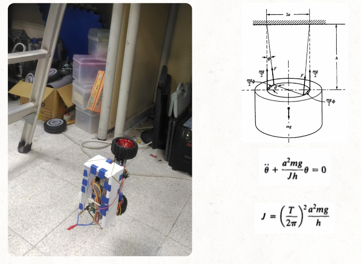
And the following is simple python code used to compute the inertia.
import numpy as np

# unit: MKS

# W is width, L is length, M is mass — fill in the measured values
W = 0.10  # width, m
L = 0.15  # length, m
M = 0.80  # mass, kg

# I is theoretical inertia, J is practical inertia

I = M/12*(W**2+L**2)
print("theoretical inertia is {}".format(I))


# calculate inertia from period T
# T is period, A is rotation radius, G is gravity, H is height — fill in the measured values
T = 1.20   # period, s
A = 0.20   # rotation radius, m
G = 9.81   # gravity, m/s^2
H = 0.30   # height, m

J = (T/2/np.pi)**2*A**2*M*G/H

print("practical inertia is {}".format(J))


error = (J-I)/I*100
print("Error is {}%".format(error))
Finally, we got the table of desired parameter.
| car | Rod Inertia | Wheel Inertia | Rod Mass | Wheel Mass | Rod Length |
|---|---|---|---|---|---|
| Big | 0.0012 | 7.8537e-05 | 0.709 | 0.087 | 0.0412 |
| Small | 5.3493e-04 | 3.4951e-05 | 0.367 | 0.042 | 0.0175 |
(units: MKS)
SIMULATION
At the simulation part, we discuss about the control model applied on the robot, there are two aspects on the model, one is state space in modern control, another one is transfer function in classical control.
STATE SPACE
After linearization with $\cos\theta \approx 1, \sin\theta \approx \theta, \dot{\theta}^2 \approx 0$
$$\begin{align} &\left((I_r+m_rL^2)[(m_w+m_r)R^2+I_w]-(m_rRL)^2\right)\ddot{\phi} \ &=[(I_r+m_rL^2)+m_rRL]\tau-(m_rRL)m_rgL\theta \ \ &\ddot{\phi}=\frac{m_r^2L^2Rg}{(m_rRL)^2-(I_r+m_rL^2)[I_w+(m_w+m_r)R^2]}\theta \ &+\frac{-(I_r+m_rL^2+m_rRL)}{(m_rRL)^2-(I_r+m_rL^2)[I_w+(m_w+m_r)R^2]}\tau \ \ &\left[(m_rRL)^2-\left((m_w+m_r)R^2+I_w\right)(I_r+m_r L^2)\right]\ddot{\theta} \ &=\left(m_rRL+(m_w+m_r)R^2+I_w\right)\tau-\left((m_w+m_r)R^2+I_w\right)m_rgL\theta \ \ &\ddot{\theta}=\frac{\left(I_w+(m_w+m_r)R^2\right)m_rgL}{\left(I_w+(m_w+m_r)R^2\right)(I_r+m_r L^2)-(m_rRL)^2}\theta \ &+\frac{-\left(m_rRL+(I_w+(m_w+m_r)R^2)\right)}{\left(I_w+(m_w+m_r)R^2\right)(I_r+m_r L^2)-(m_rRL)^2}\tau \end{align}$$
Let $\tau$ as input $u$, with states $\phi, \dot{\phi}, \theta, \dot{\theta}$, and the system is
$$\begin{align} \dot{x}&=Ax+Bu \ y&=Cx+Du \end{align}$$
where
$$\begin{align} A&= \begin{bmatrix} 0 & 1 & 0 & 0 \ 0 & 0 & \frac{m_r^2L^2Rg}{(m_rRL)^2-(I_r+m_rL^2)[I_w+(m_w+m_r)R^2]} & 0 \ 0 & 0 & 0 & 1 \ 0 & 0 & \frac{\left(I_w+(m_w+m_r)R^2\right)m_rgL}{\left(I_w+(m_w+m_r)R^2\right)(I_r+m_r L^2)-(m_rRL)^2} & 0 \end{bmatrix} \ B&= \begin{bmatrix} 0 \ \frac{-(I_r+m_rL^2+m_rRL)}{(m_rRL)^2-(I_r+m_rL^2)[I_w+(m_w+m_r)R^2]} \ 0 \ \frac{-\left(m_rRL+(I_w+(m_w+m_r)R^2)\right)}{\left(I_w+(m_w+m_r)R^2\right)(I_r+m_r L^2)-(m_rRL)^2} \end{bmatrix} \ C&= \begin{bmatrix} 1 & 0 & 0 & 0 \ 0 & 0 & 1 & 0 \end{bmatrix}\ D&= \begin{bmatrix} 0 \ 0 \end{bmatrix} \end{align}$$
TRANSFER FUNCTION
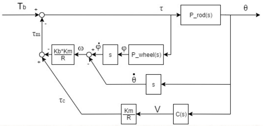
Original PID control block diagram
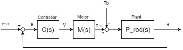
After rearrange
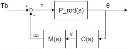
Thus get the transfer function of the controlled system

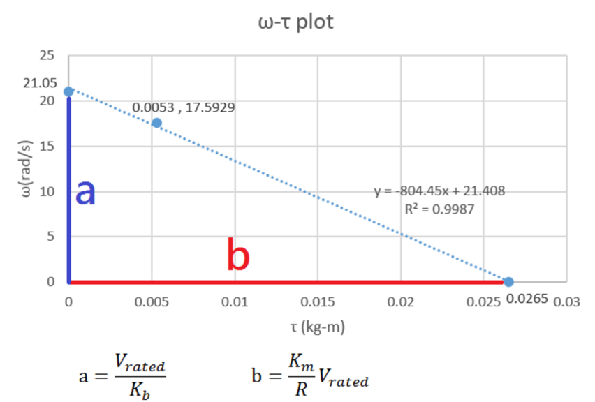
Plug in the ideal motor model to approximate the true model
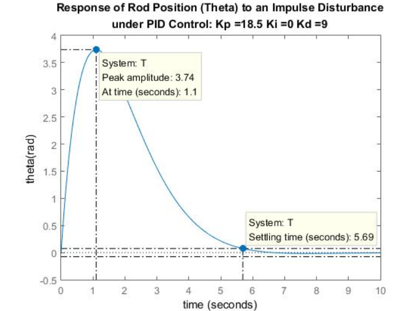
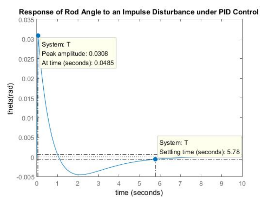
Then we have the complete transfer function
IMPLEMENTATION
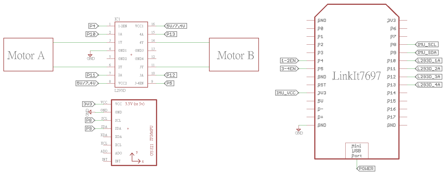
The robot car is designed in Onshape CAD and made of laser-cut acrylic board, and the main controller is LinkIt 7697 which is much more powerful than Arduino board.
To keep balance, it's needed to add an IMU (inertia measurement unit) to monitor the linear acceleration and angular velocity.
HARDWARE
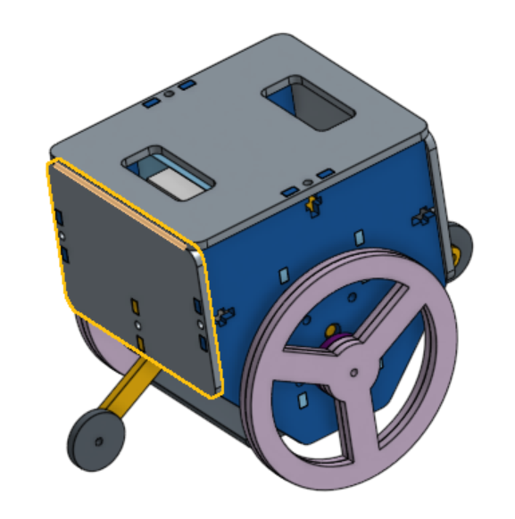
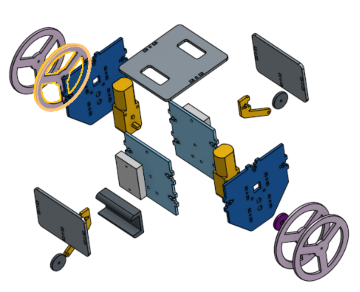
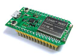
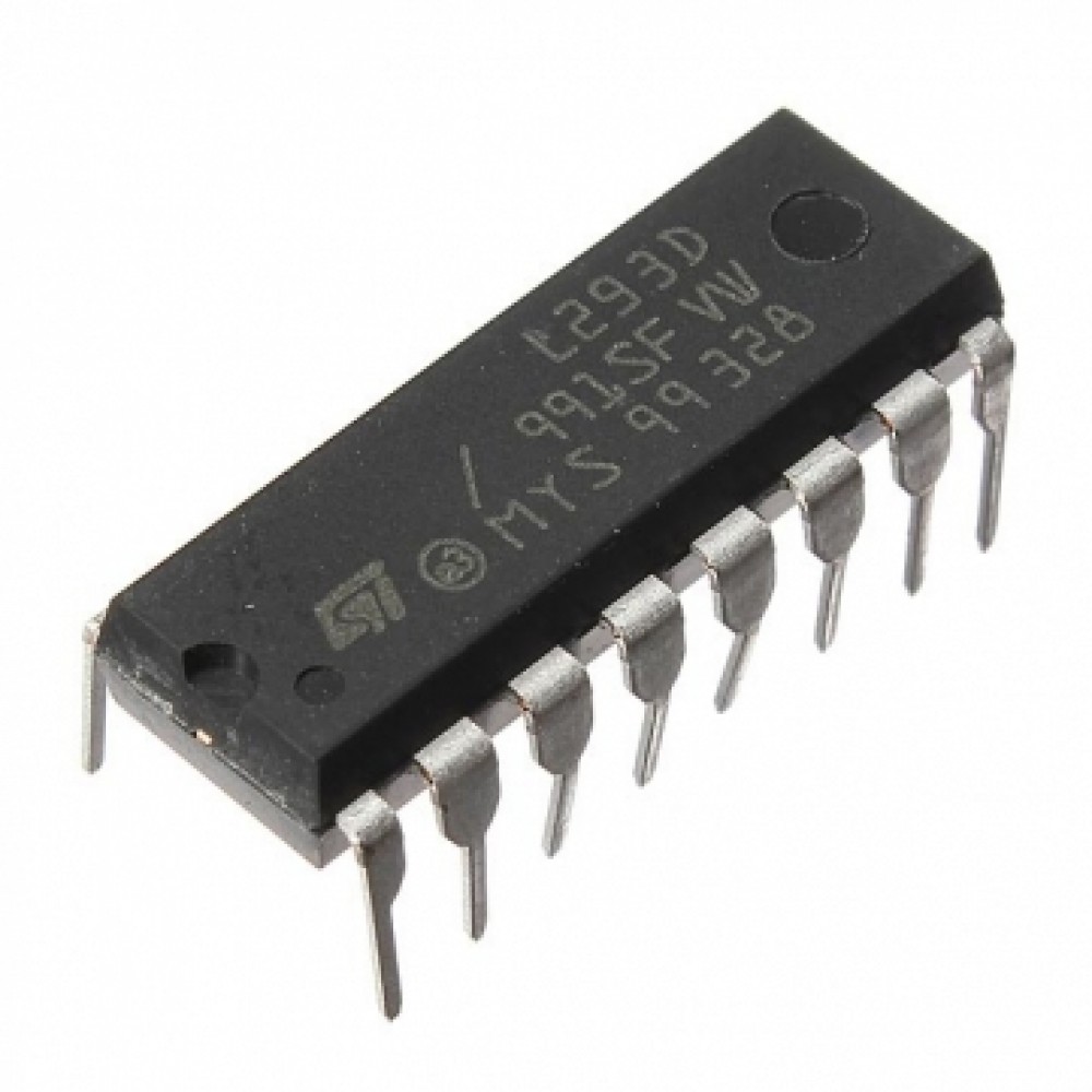
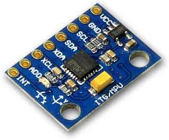
Schematics
Diagram
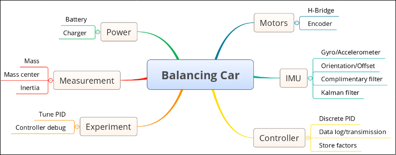
The following diagram shows the structure of the whole implementation of the robot car, some difficult works are the conversion from continuous model to discrete computation on the micro controller, and the correction of the derived angle by adding some filter like complementary filter/Kalman filter.
VIDEOS
ANALYSIS
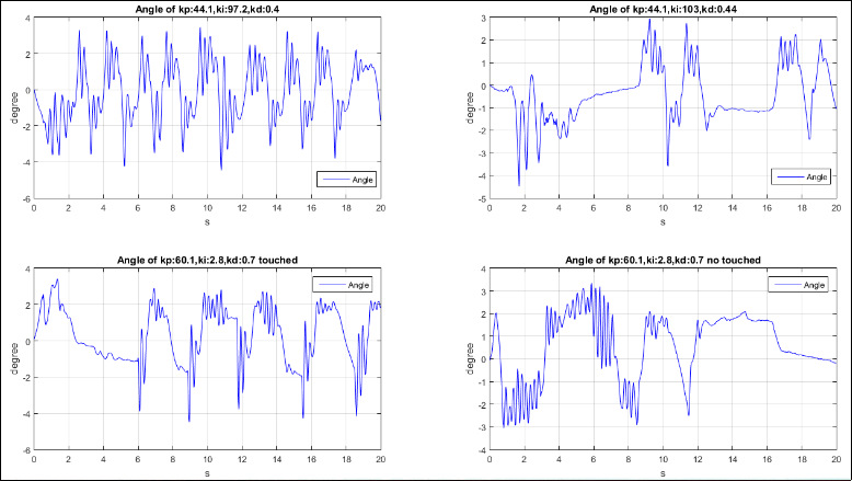
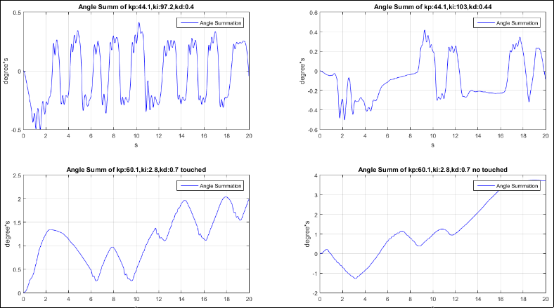
The controller 7697 has the ability to transfer the recording data to computer for analysis, the following pictures are recorded data while small car balancing with PID control.
Angle
Angle Rate
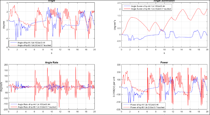
Angle Sum
FUTUREWORK: MACHINE LEARNING
Ideal vs Practical
- Continuous vs Discrete on computation
- Inaccurate IMU Angle
- Ideal Motor Model is not good enough
- Measurement Error
Since the classical method on controlling problem depends on the accuracy of physical parameter and a stable environment, maybe we can have a different way to deal with this kind of problem.
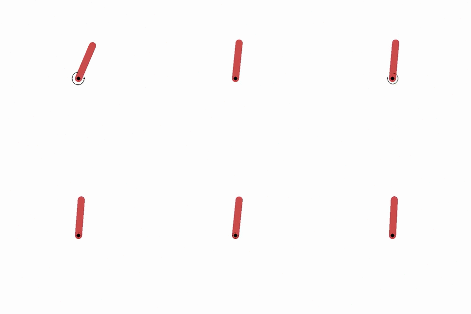
A powerful tool on dealing with continuous control problem is to use RL (Reinforcement Learning), the following simulation is used the DDPG (Deep Deterministic Policy Gradient) to balance an inverted pendulum in a custom OpenAI GYM environment.
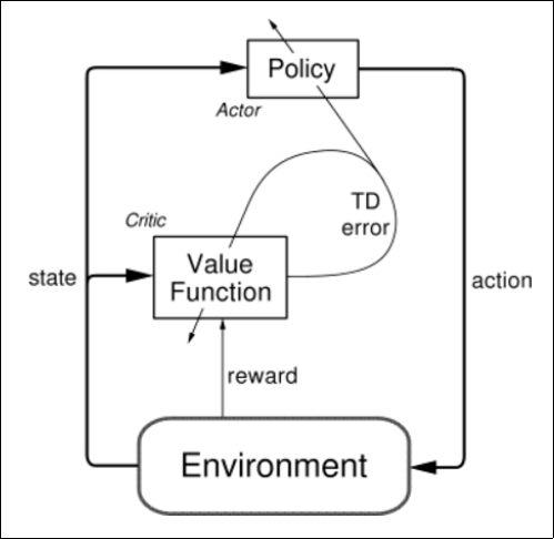
The following is the diagram for balancing car under machine learning
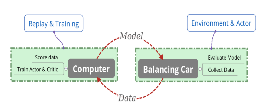
So far, there are still some works to implement the RL algorithm on the robot car, including the wireless data transmission (the C++ library is under development), and the learning environment of the robot still needs some improvement, so there's still a long way to go.
REFERENCE
MATLAB: State-Space Methods for Controller Design
MIT OCW Linear Quadratic Regulator
Continuous control with deep reinforcement learning
Measurement of moment of inertia: Katsuhiko Ogata (2004). System Dynamics (4th ed). pp.82-83 New Jersey: Pearson